Leipper and Volgenau (1972)#
This application diagnoses the Ocean Heat Content (OHC) relative to a specified isotherm depth relevant to tropical cyclone (TC) analysis and forecasting (e.g., Tropical Cyclone Heat Potential; TCHP). The application is based on that described in Leipper and Volgenau, (1972).
Configuration#
The following table provides and describes the configurable variables for the application. Note that if a Default Value is missing, the respective variable is mandatory.
Variable |
Description |
Default |
|---|---|---|
|
The depth interval for the vertical integration of the OHC in order to compute the TCHP relative to the specified isotherm; units must be identical to that of the ocean depth coordinate. |
5.0 meters |
|
The missing value to be used when interpolating the temperature variable to determine the depth of the specified isotherm; this value is assigned if the depth of the isotherm is not within the oceanic depth array values. |
|
|
The interpolation type to determine the depth of the specified isotherm. |
|
|
The isothermal level relative to which to compute the TCHP. |
\(26^{o}\text{C}\) |
|
The netCDF-formatted file path to contain the specified output variables. |
|
|
Boolean valued variable specifying whether to write the
netCDF-formatted output file defined by |
|
In addition to the above, the specified variables to be written to the
output file (output_file) can be defined by the output_vars
key. The available output variables are provided in the following
table.
Variable Name |
Description |
|---|---|
|
The relevant isotherm to compute the TCHP. |
|
The OHC from which to compute the TCHP. |
|
The TCHP. |
|
The latitude grid from which the respective gridded variables are derived. |
|
The longitude grid from which the respective gridded variables are derived. |
|
The oceanic depths from which the respective gridded variables are computed. |
|
|
|
The absolute salinity. |
An example YAML-formatted configuration file is as follows.
app_module: tcdiags.lv1972_ohc
app_class: LV1972
schema: !ENV ${TCDIAGS_ROOT}/parm/schema/tcdiags.lv1972_ohc.yaml
write_output: true
output_file: ./tcdiags.lv1972_ohc.nc
output_vars:
  tchp:
    coords: &coords2d
      - lat
      - lon
    attributes:
      description: Tropical cyclone heat potential.
  lats:
    coords: *coords2d
    attributes:
      description: Latitudes.
  lons:
    coords: *coords2d
    attributes:
      description: Longitudes.
  isotherm:
    coords: *coords2d
    attributes:
      description: Isotherm depth.
  asaln:
    coords: &coords3d
      - level
      - lat
      - lon
    attributes:
      description: Absolute salinity.
  ctemp:
    coords: *coords3d
    attributes:
      description: Conservative temperature.
  ohc:
    coords: *coords3d
    attributes:
      description: Ocean heat content.
  depths:
    coords: *coords3d
    attributes:
      description: Ocean depth.
Note that the application assumes that the environment variable
TCDIAGS_ROOT has been defined and points to the top-level
directory of the ufs_tcdiags repository clone. Further, the
output_varlist points to a YAML-formatted file containing the
variables to be written to output_file if write_output is
True. A snippet containing some of the contents written to the
netCDF-formatted file path follows.
user@host:$ ncdump -h ./tcdiags.vl1991_strflw.nc

dimensions:
        plevs = 10 ;
        lat = 192 ;
        lon = 384 ;
variables:
        int64 plevs(plevs) ;
        double lat(lat) ;
                lat:_FillValue = NaN ;
        double lon(lon) ;
                lon:_FillValue = NaN ;
        double chi(plevs, lat, lon) ;
                chi:_FillValue = 9.96920996838687e+36 ;
                chi:missing_value = 9.96920996838687e+36 ;
                chi:description = "\"The velocity potential field.\"\n" ;
                chi:name = "velocity potential" ;
                chi:units = "meters^2/second" ;
        double divg(plevs, lat, lon) ;
                divg:_FillValue = 9.96920996838687e+36 ;
                divg:missing_value = 9.96920996838687e+36 ;
                divg:description = "\"The total divergence field.\"\n" ;
                divg:name = "divergence" ;
                divg:units = "1/second" ;
Running the Application#
The TC steering flow application can be executed using a variety of methods. Each is described below.
Terminal#
The TC steering flow application may be executed within an supporting environment as follows.
user@host:$ export PYTHONPATH="/path/to/ufs_tcdiags/ush":"${PYTHONPATH}"
user@host:$ cd /path/to/ufs_tcdiags/scripts
user@host:$ ./compute_tcdiags.py --help

Usage: compute_tcdiags.py [-h] [-tcmsi] [-tcpi] [-tcstrflw] yaml

Tropical cyclone diagnostics computation(s) application interface.

Positional Arguments:
  yaml        YAML-formatted tropical cyclone diagnostics configuration file.

Optional Arguments:
  -h, --help  show this help message and exit
  -tcmsi      YAML-formatted file containing the TC multi-scale intensity application configuration.
  -tcpi       YAML-formatted file containing the TC potential intensity application configuration.
  -tcstrflw   YAML-formatted file containing the TC steering application configuration.

user@host:$ ./compute_tcdiags.py /path/to/ufs_tcdiags/parm/tcdiags.demo.yaml -tcstrflw
Jupyter Notebook#
The TC steering flow application can also be executed from within a Jupyter notebook as follows.
user@host:$ export PYTHONPATH="/path/to/ufs_tcdiags/jupyter":"/path/to/ufs_tcdiags/ush":"${PYTHONPATH}"
user@host:$ cd /path/to/ufs_tcdiags/jupyter/notebooks
user@host:$ /path/to/jupyter notebook tcdiags.vl1991_strflw.ipynb
This action behaves as the terminal instance for the application (above) but is executed from within the respective Jupyter notebook.
Docker Container#
The TC steering flow application may be executed within an appropriate Docker container as follows.
user@host:$ /path/to/docker run -v /path/to/ufs_tcdiags:/home/ufs_tcdiags -it ghcr.io/henrywinterbottom-noaa/ubuntu20.04.ufs_tcdiags:latest
user@host:$ export PYTHONPATH="/home/ufs_tcdiags/ush":"${PYTHONPATH}"
user@host:$ cd /home/ufs_tcdiags/scripts
user@host:$ ./compute_tcdiags.py --help

Usage: compute_tcdiags.py [-h] [-tcmsi] [-tcpi] [-tcstrflw] yaml

Tropical cyclone diagnostics computation(s) application interface.

Positional Arguments:
  yaml        YAML-formatted tropical cyclone diagnostics configuration file.

Optional Arguments:
  -h, --help  show this help message and exit
  -tcmsi      YAML-formatted file containing the TC multi-scale intensity application configuration.
  -tcpi       YAML-formatted file containing the TC potential intensity application configuration.
  -tcstrflw   YAML-formatted file containing the TC steering application configuration.

user@host:$ ./compute_tcdiags.py /home/ufs_tcdiags/parm/tcdiags.demo.yaml -tcstrflw
Jupyter Notebook Within a Docker Container#
Similar to the Jupyter notebook and Docker container examples above, the Jupyter notebook can also be launched from within the Docker container. This can be accomplished as follows.
user@host:$ /path/to/docker run -v /path/to/ufs_tcdiags:/home/ufs_tcdiags -p 8888:8888 -it ghcr.io/henrywinterbottom-noaa/ubuntu20.04.ufs_tcdiags:latest
user@host:$ export PYTHONPATH="/home/ufs_tcdiags/ush":"/home/ufs_tcdiags/jupyter":"${PYTHONPATH}"
user@host:$ cd /path/to/ufs_tcdiags/jupyter/notebooks
user@host:$ /path/to/jupyter notebook --ip=0.0.0.0 --port=8888 --no-browser --allow-root tcdiags.vl1991_strflw.ipynb
The above action will provide the user a local HTML path and an associated token as follows.
To access the server, open this file in a browser:
    file:///root/.local/share/jupyter/runtime/jpserver-21362-open.html
Or copy and paste one of these URLs:
    http://5186640b39b0:8889/tree?token=abcdefghijklmnopqrstuvwxwy0123456789ABCDEFGHIJKL
    http://127.0.0.1:8889/tree?token=abcdefghijklmnopqrstuvwxwy0123456789ABCDEFGHIJKL
Copy the paste the token attribute that begins with
http://127.0.0.1:8889 into a web browser address bar and execute
the respective Jupyter notebook as described above.
Example Results#
The following example is computed from a nominally 1.0-degree ERA5 analysis valid 0000 UTC 01 October 2016.
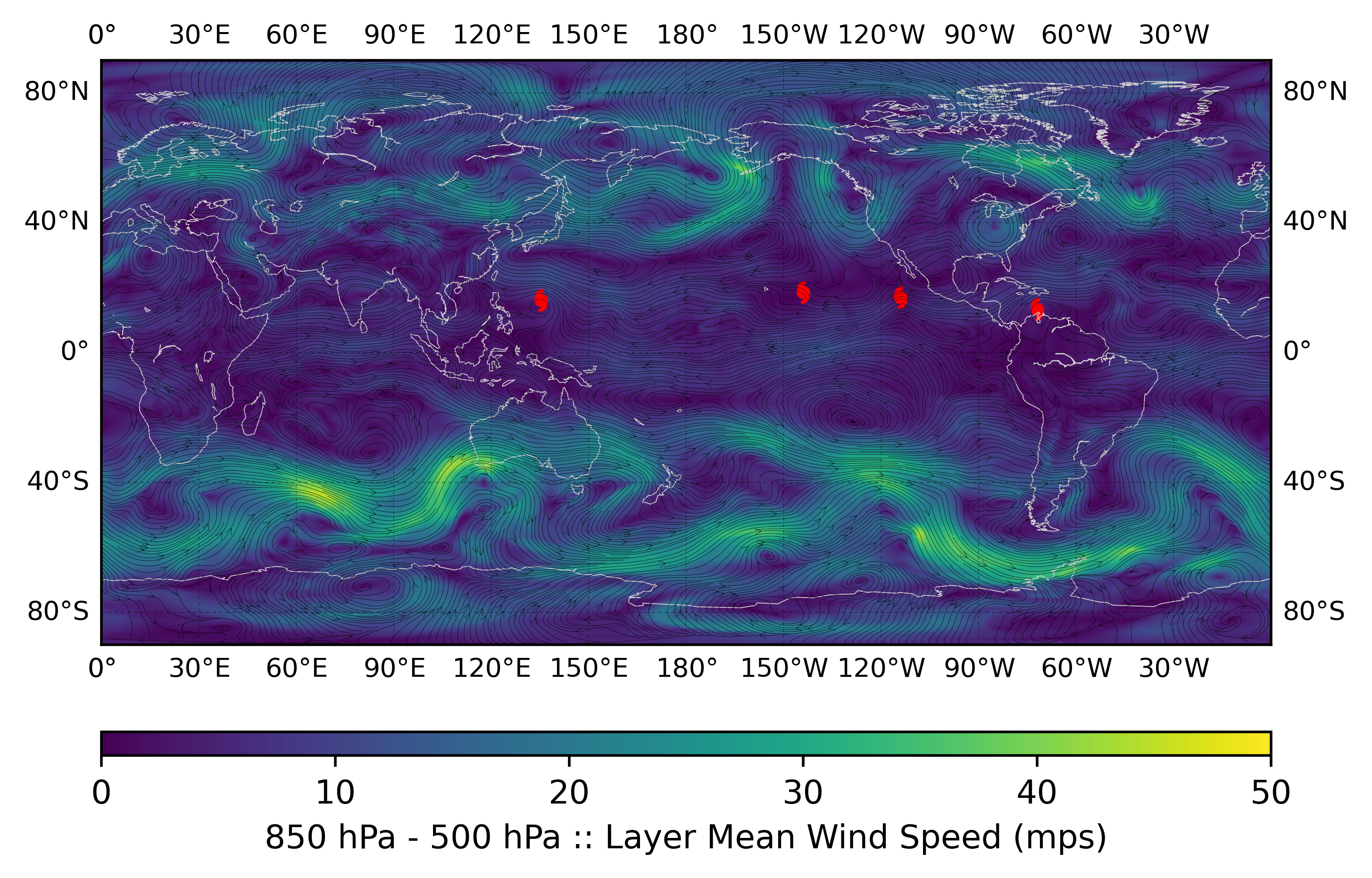
|
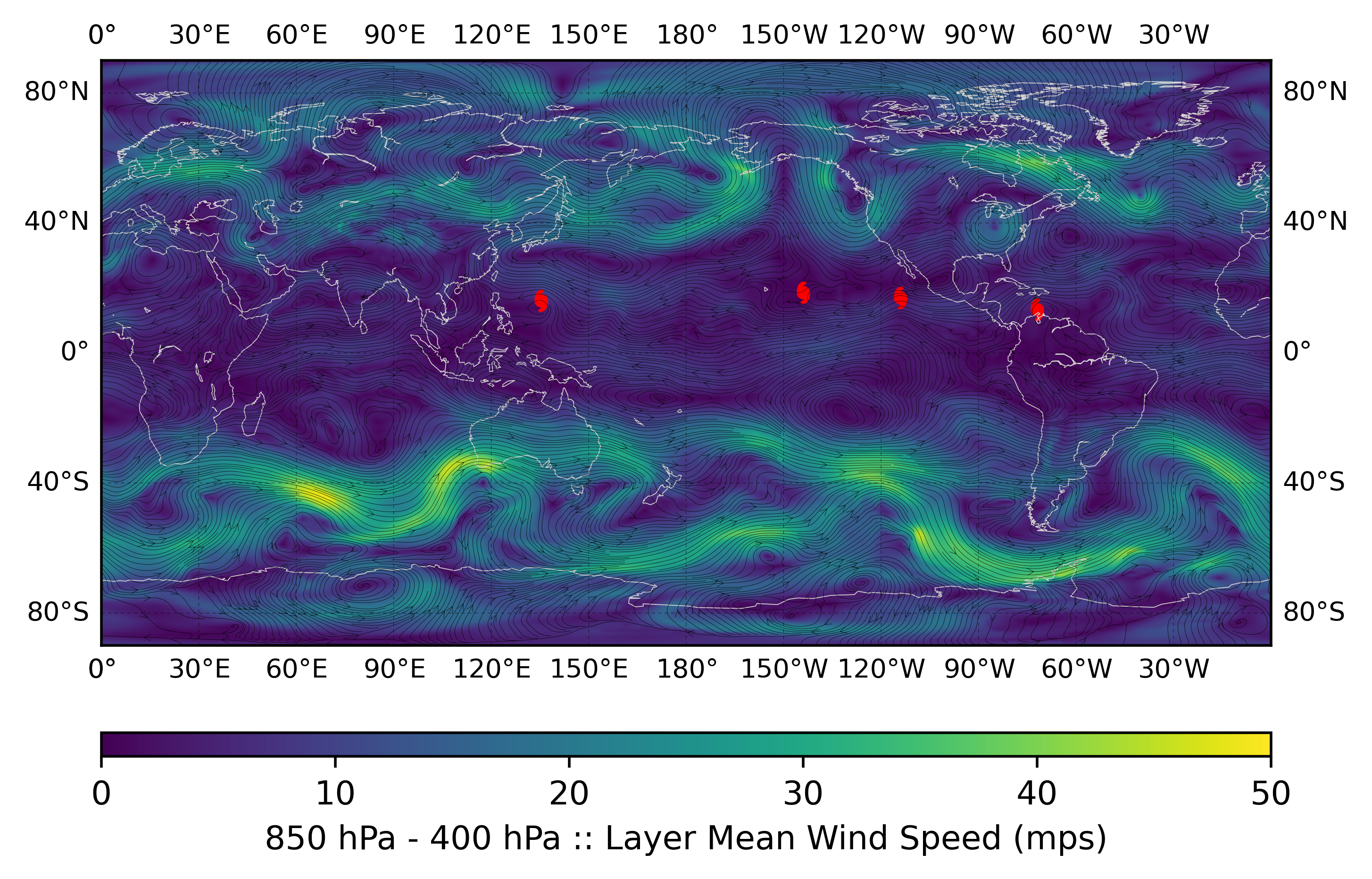
|
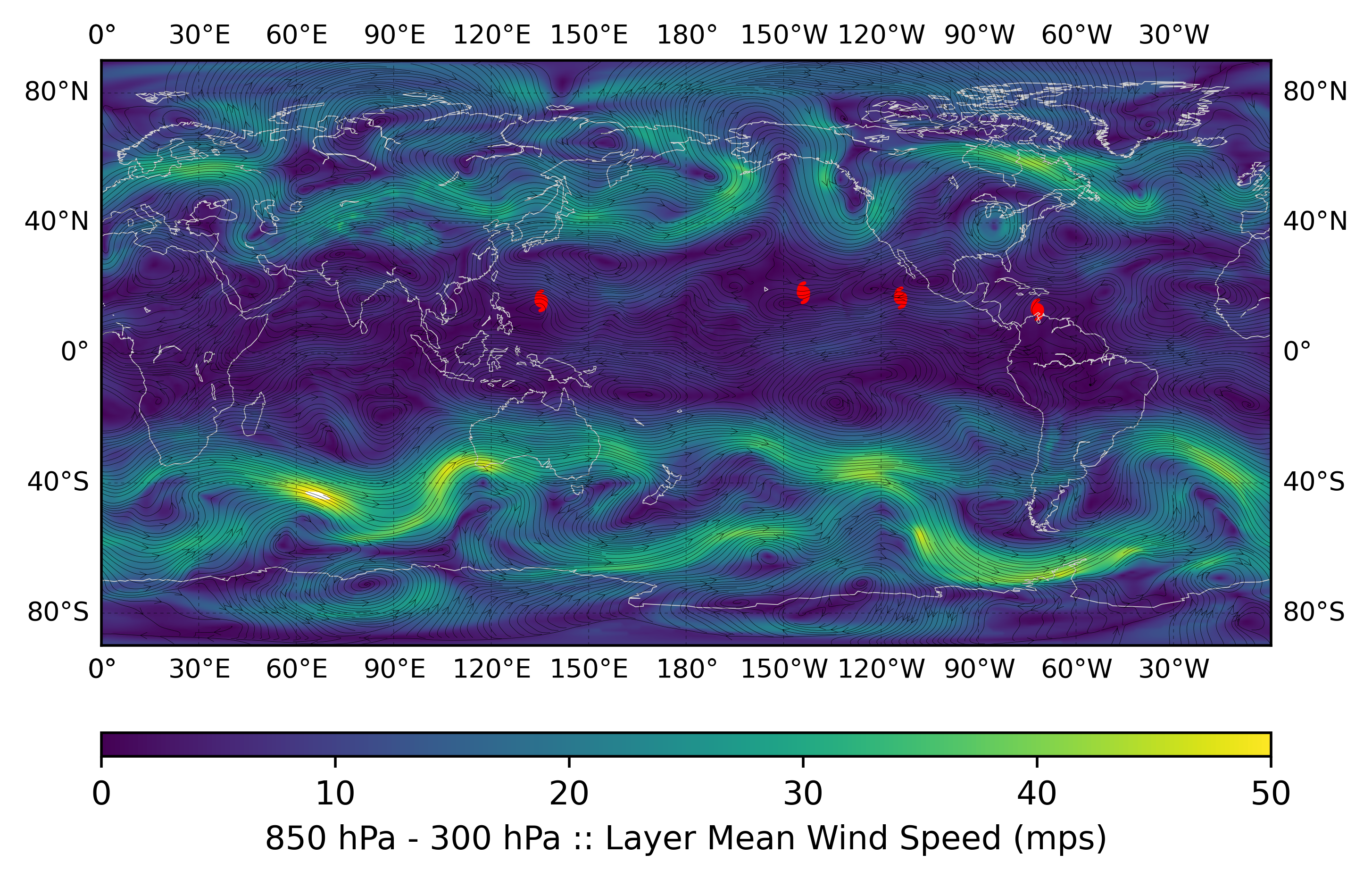
|
The layer-mean winds with respect to the intensity ranges illustrated by Figure 2 of Velden and Leslie, (1991) are shown above for the 850- to 500-hPa (top), 850- to 400-hPa (center), and 850- to 300-hPa (bottom). The TC locations, valid for 0000 UTC 01 October 2016, are denoted by the respective red symbols.